Version 2.00Ok guys and girls, this is a guide/reference for using the Ti-nspire for Specialist Maths. It will cover the simplest of things to a few tricks. This guide has been written for Version 3.1.0.392. To update go to
http://education.ti.com/calculators/downloads/US/Software/Detail?id=6767Any additions or better methods are welcomed. Also let me know if you spot any mistakes.
Guide to Using the Ti-nspire for METHODS - The simple and the overcomplicated: http://www.atarnotes.com/forum/index.php?topic=125386.msg466347#msg466347
Printer Friendly PDF version: http://www.atarnotes.com/?p=notes&a=feedback&id=661NOTE: There is a mistake in the printable version. Under the shortcut keys the highlighting should read "Copy: Ctrl left or right to highlight, [SHIFT (the one with CAPS on it)] + [c]"Simple things will have green headings, complicated things and tricks will be in red. Firstly some simple things. Also Note that for some questions, to obtain full marks you will need to know how to do this by hand. DONT entirely rely on the calculator. Remember this should help speed through those Multiple Choice and to double check your answers for Extended Respons quickly.
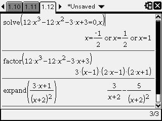
Solve, Factor & ExpandThese are the basic functions you will need to know.
Open Calculate (A)
Solve: [Menu] [3] [1] (equation, variable)|Domain
Factor: [Menu] [3] [2] (terms)
Expand: [Menu] [3] [3] (terms)
 Vectors
These way the Ti-nspire handles vectors is to set them up like a 1 X 3 matrix. E.g. The vector 2
i+2
j+1
k would be represented by the matrix

You can enter a matrix by pressing [ctrl] + ["x"], then select the 3 X 3 matrix and enter in the appropriate dimensions.
Its easier to work with the vectors if you define them. E.g. [Menu] [1] [1] a =
The functions that can be applied to the vectors are:
Unit Vector: [Menu] [7] [C] [1] - unitV(

)
Dot Product: [Menu] [7] [C] [3] dotP(

,
)
Magnitude: type "norm()" norm(
)
E.g.
a=2
i+2
j+
k,
b=6
i+2
j-16
k, Find the Unit vector of
a and
a.
b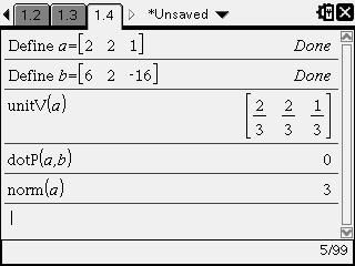
E.g.
a and
b are perpendicular
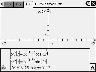
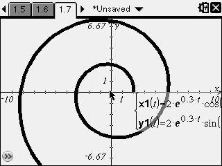
Graphing Vectors EquationsNormally expresses as a function of t. Graphed as parametric equations. Select the graph entry bar, [ctrl] + [Menu] [2:Graph Type] [2:Parametric]
Enter in the
i coefficient as x1(t) and the
j coefficient as x2(t)
e.g. Graph
=2e^{0.3t}\cos(2t)\mathbf{\vec{i}}+2e^{0.3t}\sin(2t)\boldsymbol{\vec{j}})
 Complex Numbers
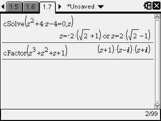
 There are two important functions related to complex numbers. They work the same as the original functions, but will give complex solutions aswell.
cSolve: [Menu] [3] [C] [1]
cFactor: [Menu] [3] [C] [1]
E.g. Solve

for z and factorise

 Quicker Cis(θ) Evaluations
1. Define ([Menu] [1] [1]) cis(θ)=\cos(θ)+
i\sin(θ)
2. Simply plug in the value of theta
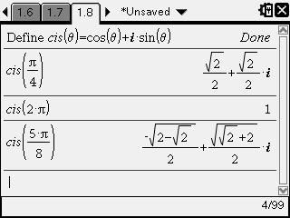 Finding Arguments
1. Use the angle function (i.e. find it in the catalogue of type angle(*)
E.g. Find the Argument of

 Defining Domains
While graphing or solving, domains can be defined by the addition of |lowerbound<x<upperbound
The less than or equal to and greater than or equal to signs can be obtained by pressing ctrl + < or >
e.g. Graph

for

Enter
=x^2 |-2<x\leq 1)
into the graphs bar

This is particulary useful for fog and gof functions, when a domain is restriced, the resulting functions domain will also be restricted.
E.g. Find the equation of
)
when
=x^2,x \in(-2,1] )
and
=2x+1,x\in R )
1. Define the two equations in the Calulate page. [Menu] [1] [1]

2. Open a graph page and type, f(g(x)) into the graph bar

The trace feature can be used to find out the range and domain. Trace: [Menu] [5] [1]
Here
=(2x+1)^{2})
where the Domain = (-1.5,1] and Range =[0,4)
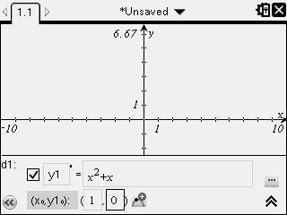
Completing the SquareThe easy way to find the turning point quickly. The Ti-nspire has a built in function for completing the square.
[Menu] [3] [5] - (function,variable)
e.g. Find the turning point of


So from that the turning point will be at (-2,1)
Easy Maximum and MinimumsIn the newer version of the Ti-nspire OS, there are functions to find maximum, minimums, tangent lines and normal lines with a couple of clicks, good for multiple choice, otherwise working would need to be shown. You can do some of these visually on the graphing screen or algebraically in the calculate window.
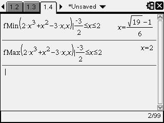
Maximums: [Menu] [4] [7] (terms, variable)|domain
Minimums: [Menu] [4] [8] (terms, variable)|domain
E.g. Find the values of x for which

has a maxmimum and a minimum for

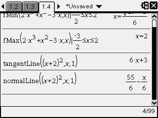
Tangents at a point: [Menu] [4] [9] (terms, variable, point)
Normals at a point: [Menu] [4] [A] - (terms, variable, point)
E.g. Find the equation of the tangent and the normal to the curve
^{2})
when

.
 Visualisation of Addition of Ordinates
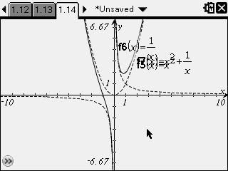
Graph f(x) and g(x), then graph f(x)+g(x)
E.g. Graph

Then
=x^{2}, g(x)=\frac{1}{x})
 Finding Vertical Asymptotes
Vertical Asymptotes occur when the function is undefined at a given value of x, i.e. when anything is divided by 0. We can manipulate this fact to find vertical asymptotes by letting the function equal

and solving for x.
e.g. Find the vertical asymptotes for
,x\in[-2\pi,2\pi])

So for
there is a vertical asymptotes at

and

Dont forget to find those other non-vertical asymptotes too.
The x-y Function TestEvery now and then you will come across this kind of question in a multiple choice section.
If
+f(y)=f(xy))
, which of the following is true?
A.
=x^2)
B.
=\ln(x) )
C.
= \frac{1}{x} )
D.
=x)
E.
=(x+2)^2)
You could do it by hand or do it by calculator. The easiest way is to define the functions and solve the condition for x, then test whether the option is true. If true is given, it is true otherwise it is false.

So option B is correct.
The Time Saver for DerivativesBy defining, f(x) and then defining df(x)= the derivative, you wont have to continually type in the derivative keys and function. It also allows you to plug in values easily into f(x) and f(x).
Derivative: [Menu] [4] [1]
E.g. Find the derivative of

Define f(x), then define df(x)

The same thing can be done for the double derivative.

Just remember to redefine the equations or use a different letter, e.g. g(x) and dg(x)
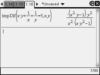
Implicit Differentiation [Menu] [4] [E] impDif(equation, variable 1, variable 2)
E.g. Differentiate

with respect to x.
 Solving For Coefficients Using Definitions of Functions
 Instead of typing out big long strings of equations and forgetting which one is the antiderivative and which one is the original, defined equations can be used to easily and quickly solve for the coefficients.
E.g. An equation of the form

cuts the x-axis at (-2,0) and (2,0). It cuts the y-axis at (0,1) and has a local maximum when

. Find the values of a, b, c & d.
1. Define
=ax^3+bx^2+cx+d)
(Make sure you put a multiplication sign between the letters)
2. Define the derivative of the f(x) i.e. df(x)
3. Use solve function and substitute values in, solve for a, b, c & d.


So

and

and the equation of the curve is
=\frac{1}{2}x^3-\frac{1}{4}x^2-2x+1) Deriving Using the Right Mode
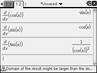
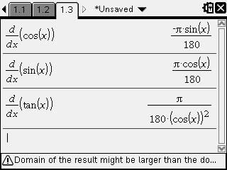
Deriving Using the Right Mode The derivative of circular functions are different for radians and degrees. Remember to convert degrees to radians and be in radian mode, as the usual derivatives that you learn e.g.
)=\cos(x))
are in radians NOT degrees.
RADIAN MODE DEGREES MODE
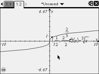
 Getting Exact Values On the Graph Screen
Now for what you have all been dreaming of. Exact values on the graphing screen. Now the way to do this is a little bit annoying.
1. Open up a graph window
2. Plot a function e.g.
=\sqrt[3]{x})
3. Trace the graph using [Menu] [5] [1]
4. Trace right till you hit around 0.9 or 1.2 and click the middle button to plot the point.
5. Press ESC
6. Move the mouse over the x-value and click so that it highlights, then move it slightly to the right and click again. Clear the value and enter in

.
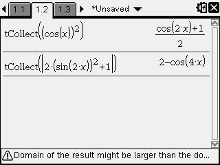
Using tCollect to simplify awkward expressions Sometimes the calculator wont simplify something the way we want it to. tCollect simplifies expressions that involves trigonometric powers higher than 1 or lower than -1 to linear trigonometric expressions.
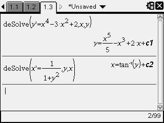
 Differntial Equation Solver
[Menu] [4] [D] DeSolve(equation, variable on bottom, variable on top)
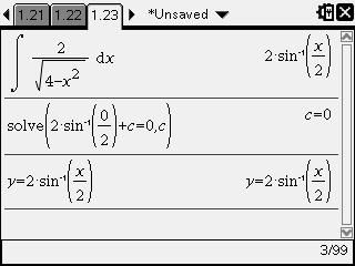
 Integrals
[Menu] [4] [3]
E.g. If find

if

and y=0 when x=0
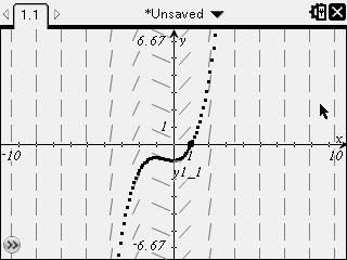
 Plotting Differential Equations + Slope Fields
Firstly you will need to open a graphing screen.
Then you need to setup up the mode for differential equations. This can be done in two ways:
A. Select the graph entry bar and press [Ctrl] [Menu] then select [2] (Graph Type) [6] (Differential Equation)
or
B. [Menu] [3] [6]
Now the interface comes up.
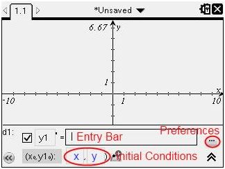
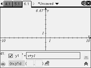
NOTE 1: When entering y in the bar, you will have to enter y1.
NOTE 2: If you want to plot a second differential equation that is not related to the first, you will need to either, open a new document (not just a graphing screen, for some reason the original equation that you plotted will be shown again) or clear out all the differential equations in the graph entry bar (i.e. y1, y2...) or open a new problem in the current document by pressing
[Ctrl] [Home] [4] [1] [2]e.g. Sketch the slope field
)
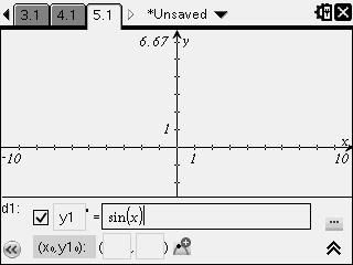
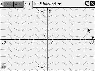
e.g. Sketch the slope field of

for

NOTE: Make sure you use y1
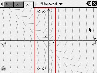
You will only need to draw the lines in the red box since
if you draw the unrequited lines you may lose marks
e.g. Sketch the slope field for

with initial conditions x=1 when y=0
Dont forget a slope field should have a table of values with it.
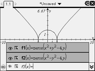
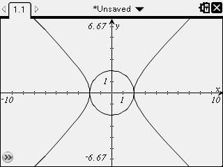
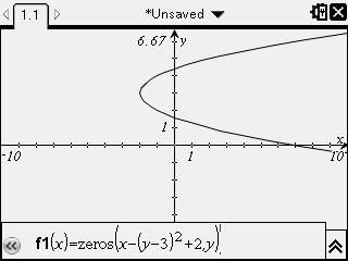
Graphing Circles, Elipses, Hyperbolas in 1.5 easy stepsThis allows you to plot equations in their zero form easily without having to rearrange for y and forming two (or more) equations.
Step 0: Firstly what you have to is rearrange the equation so that it equals 0.
e.g.

becomes


becomes

^{2}-2)
becomes
^{2}+2=0)
Now remove the

part
Step 1: Enter in the graph bar zeros(equation, dependent variable)
 Shortcut Keys
Copy: Ctrl left or right to highlight, [SHIFT (the one with CAPS on it)] + [c]
Paste: [Ctrl] + [v]
Insert Derivative: [CAPS] + ["-"]
Insert Integral: [CAPS] + ["+"]
∞: [Ctrl] + [
i]
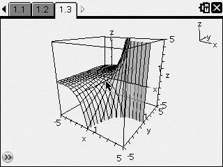
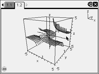
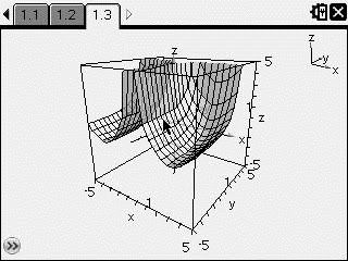
Thanks to Jane1234 & duquesne9995 for the shortcut keys. Thanks to vgardiy for the real easy sketching of equations in their zero form.Remember you can always do other funs things like 3-D graphs. Enjoy. Yey 800
th post.